Statistical Comparison of Various Dayside Magnetopause Reconnection X-line Prediction Models


Ramiz A. Qudsi,
Brian Walsh, J. Broll, Emil Atz, Stein Haaland
Boston University, Los Alamos National Lab, Max-Planck Institute
*(qudsira@bu.edu)
1 2 1 3
1, *
1 2 3
Qudsi (qudsira@bu.edu)
https://sites.bu.edu/bwalsh
Center for Space Physics
Space Physics and Technology Lab


Outline:
- Magnetic Reconnection
- X-lines
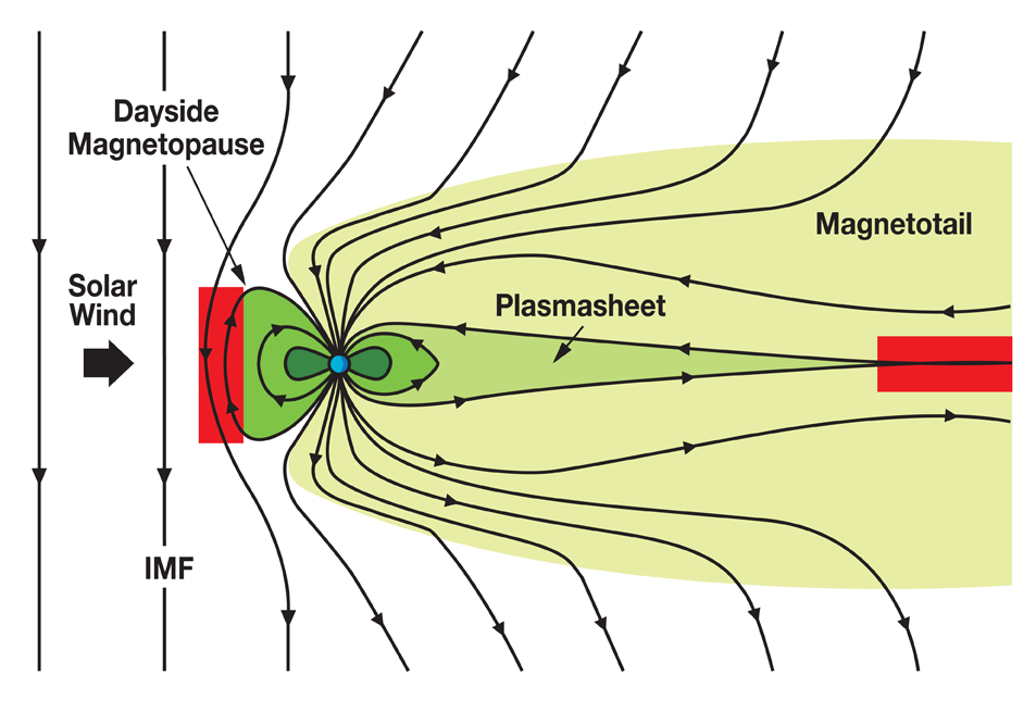
- Region of interest
- Location of x-line
- Different models
- Data
- Results
- Discussions
Qudsi (qudsira@bu.edu)
The BASICS
Qudsi (qudsira@bu.edu)
Source: NASA
Qudsi (qudsira@bu.edu)
[Broll et al., 2017]
Source: wikipedia
Qudsi (qudsira@bu.edu)
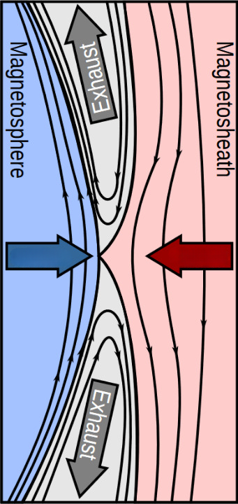
Inflow
Inflow
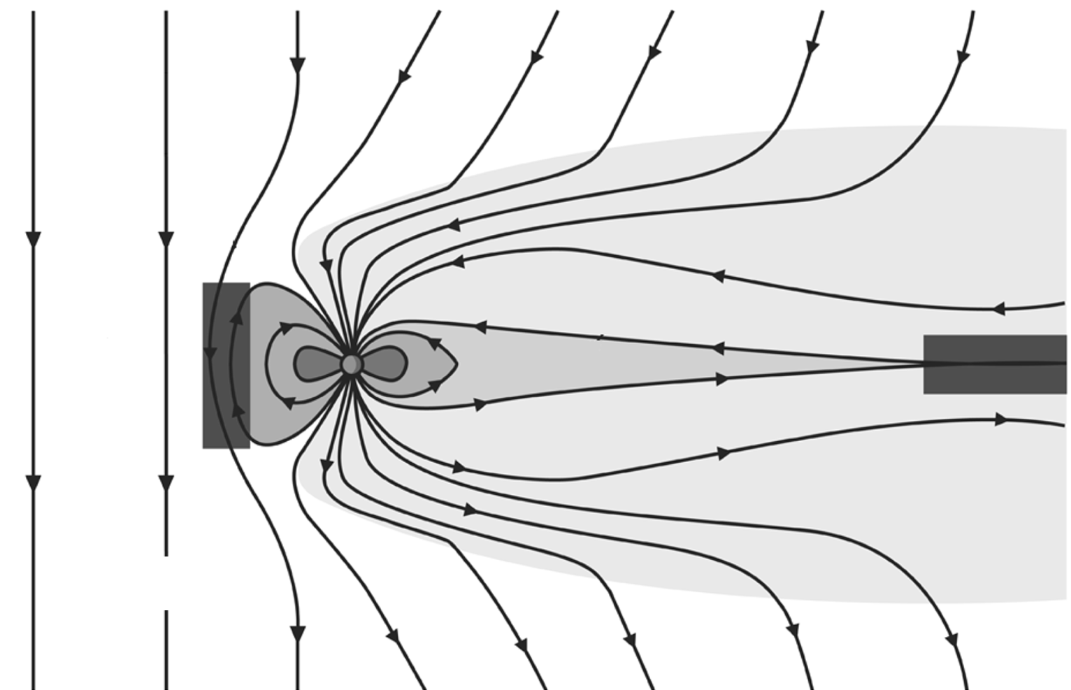
Region of interest:
Qudsi (qudsira@bu.edu)
Qudsi (qudsira@bu.edu)
Why Magnetic Reconnection?
Need to work on something!
Why not?
Ubiquitous nature of reconnection
Energy dynamics
Dynamo effect
Qudsi (qudsira@bu.edu)
Reconnection models
Qudsi (qudsira@bu.edu)
Questions regarding reconnection:
- Where?
- When?
- How fast?
- How long?
Qudsi (qudsira@bu.edu)
Classical picture:
- Anti-parallel reconnection
- Crooker-1979
- Component reconnection
- Uniform, out of plane guide field
- Sonnerup-1974, Gonzalez and Mozer-1974
- Equal and opposite component of reconnecting fields
- Cowley-1976
- Uniform, out of plane guide field
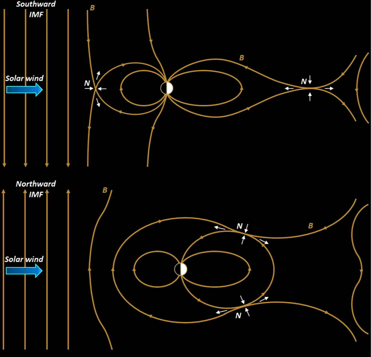
[Dungey-1961, Trattner-2021]
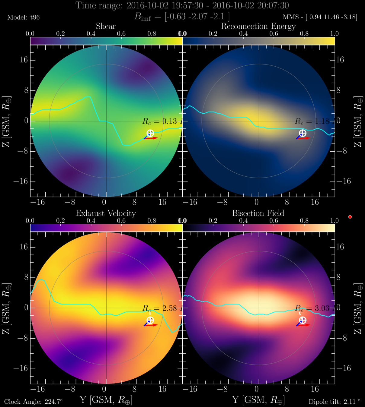
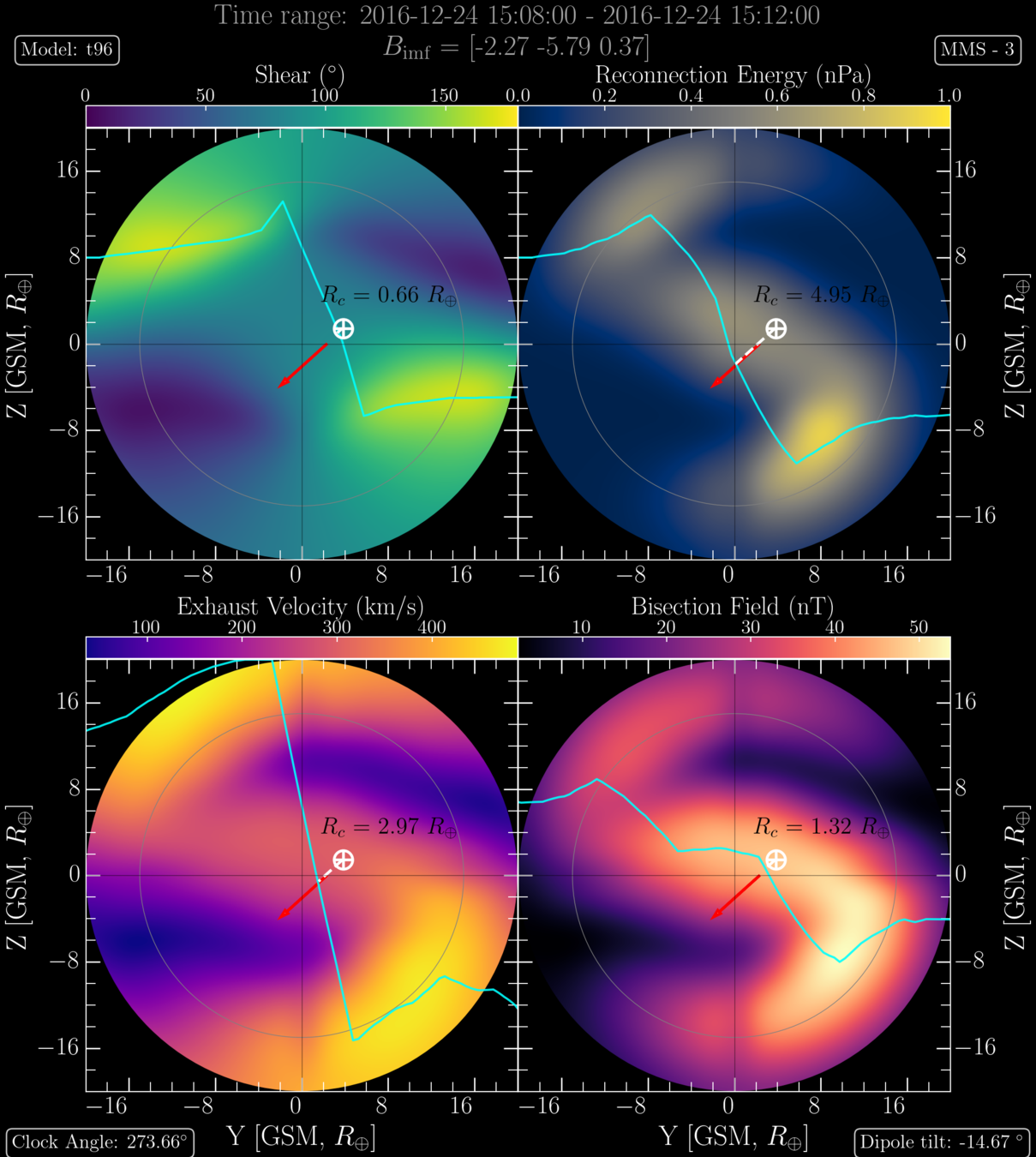
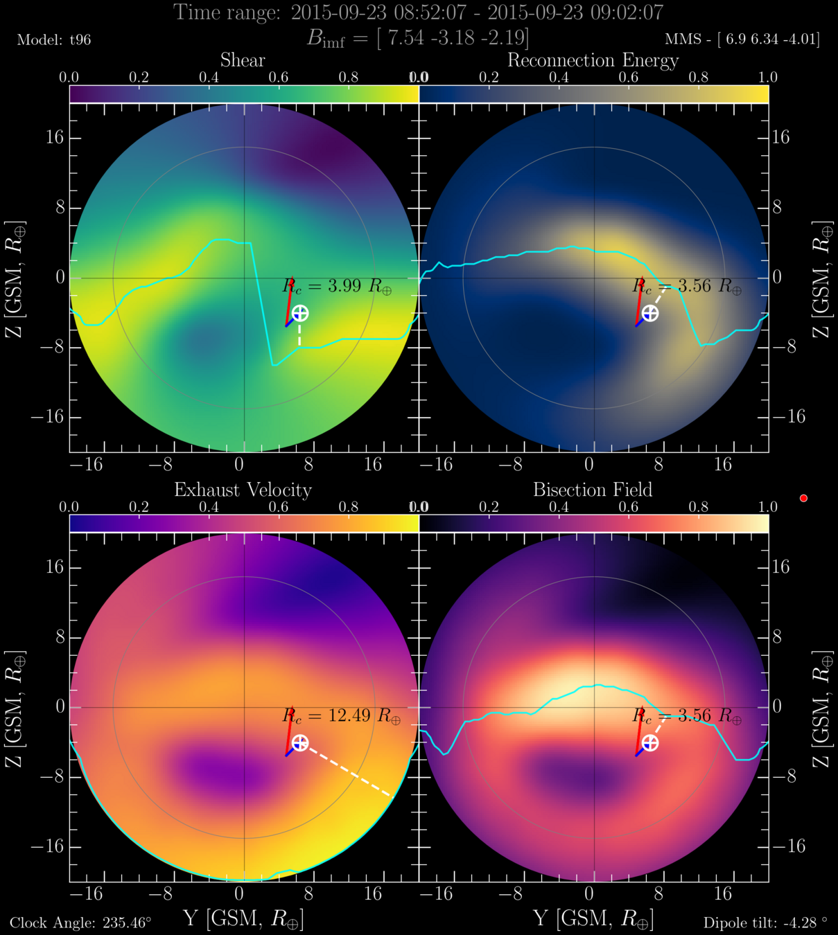
A slightly more modern picture
Local field bisection [Moore et al., 2002]
Maximum exhaust speed [Swisdak and Drake, 2007]
Maximum magnetic shear [Trattner et al., 2007]
Maximum reconnecting field energy [Hesse et al., 2013]
Qudsi (qudsira@bu.edu)
Reconnection occurs where some parameter is maximized
Maximum Current Density [Alexeev et al., 1998]
Magnetic shear [Trattner et al., 2007]:
Local field bisection [Moore et al., 2002]:
Reconnection field energy [Hesse et al., 2013]:
Exhaust speed [Swisdak and Drake, 2007]:
sh: magnetosheath
msp: magnetosphere
Location of x-line: Models
Qudsi (qudsira@bu.edu)
: unit vector normal to X-line
DATA
Qudsi (qudsira@bu.edu)
Data:
Solar
Wind
OMNI
Cooling-2001
Magnetosheath
Magnetopause
Shue-1998
T-96 + IGRF
Magnetospheric Fields
Qudsi (qudsira@bu.edu)
Data
Solar Wind data: OMNI (propagated to the magnetopause)
Magnetosheath data: MMS (FPI and FGM)
Magnetospheric magnetic field: Models (T96 and IGRF)
Magnetosheath magnetic field: Models (Cooling model)
Qudsi Center for Space Physics, BU qudsira@bu.edu
GSM coordinate system
y
z
x
Methodology
Qudsi (qudsira@bu.edu)
Methodology
- Look at the instances when MMS observed a jet reversal while crossing the magnetopause.
Qudsi (qudsira@bu.edu)
Methodology
- Look at the instances when MMS observed a jet reversal while crossing the magnetopause.
Qudsi (qudsira@bu.edu)
[Broll et al., 2017]
Qudsi (qudsira@bu.edu)
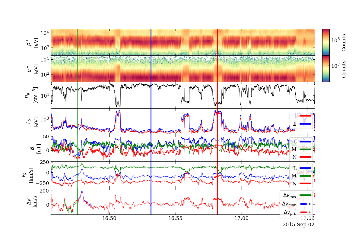
Magnetosheath
Magnetosphere
MMS data (FPI & FGM)
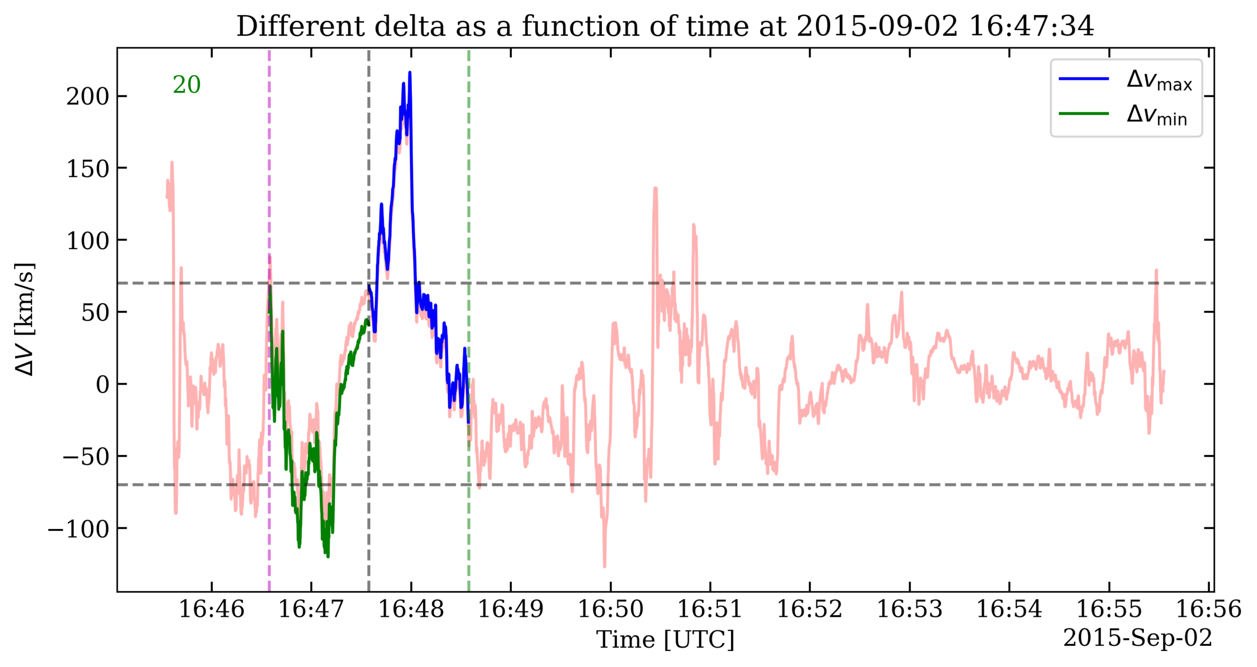
Jet Center
[Qudsi et al., 2023, in Prep]
Methodology
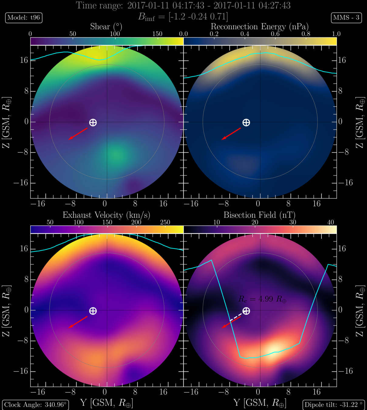
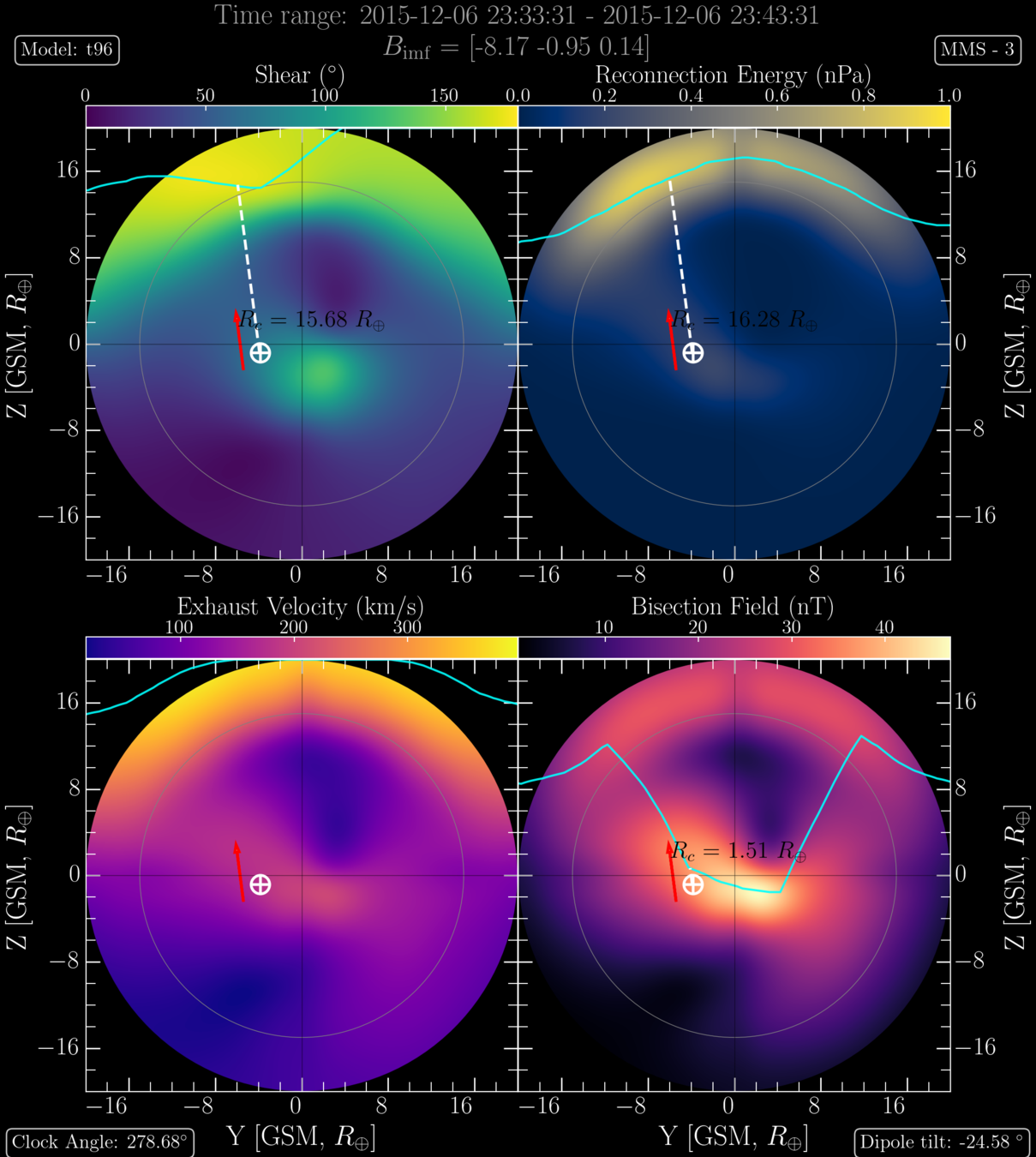
- For the observed parameters of IMF, Magnetosheath and Magnetosphere and Magnetopause find the model predicted x-line locations.
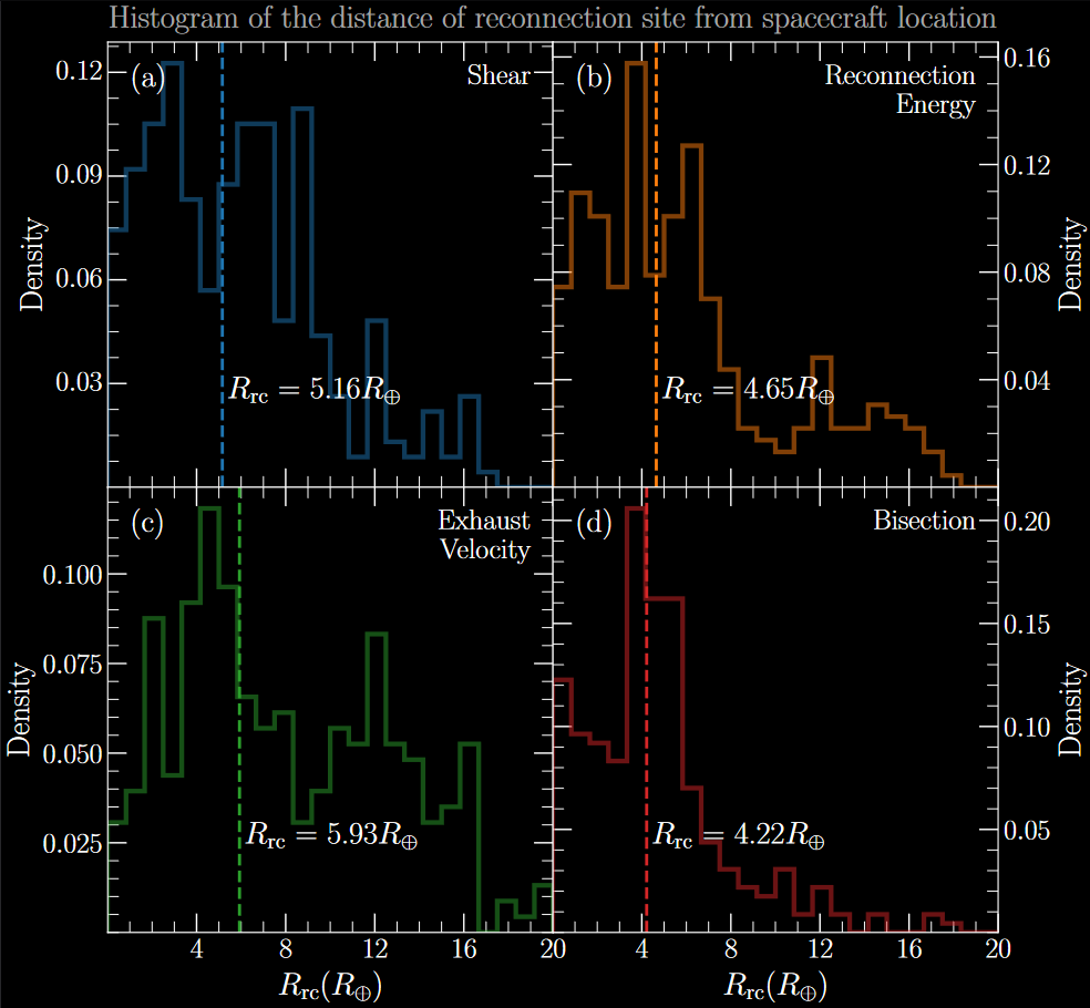
- Find the distance of x-line from MMS, along the magnetopause, for different models.
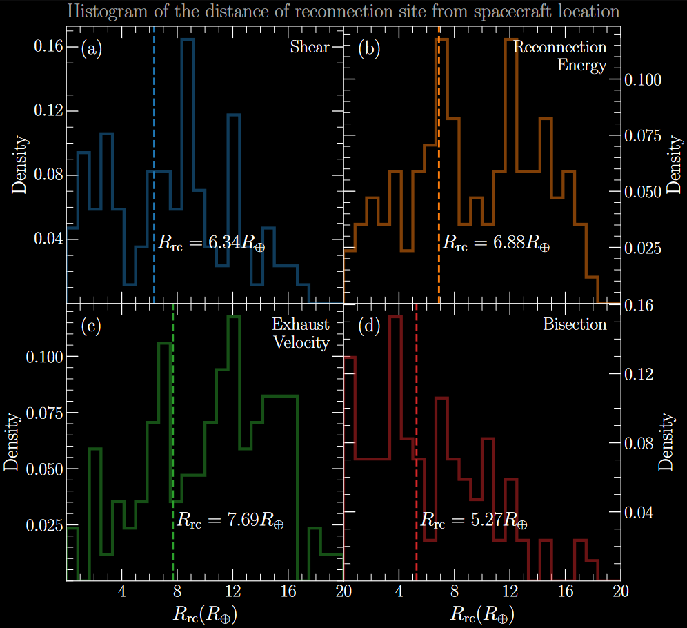
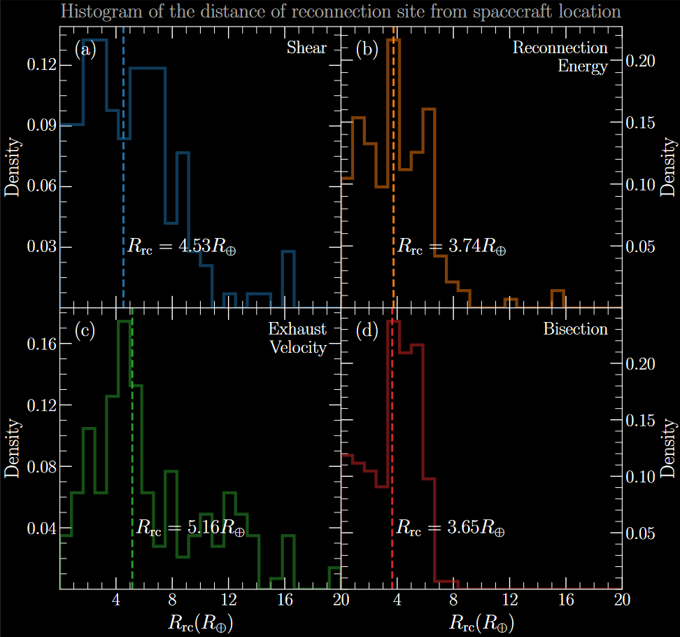
- Look at the statistical distribution of distances (histogram etc.) for different models.
Qudsi (qudsira@bu.edu)
- Look at the instances when MMS observed a jet reversal while crossing the magnetopause.
RESULTS
Qudsi (qudsira@bu.edu)
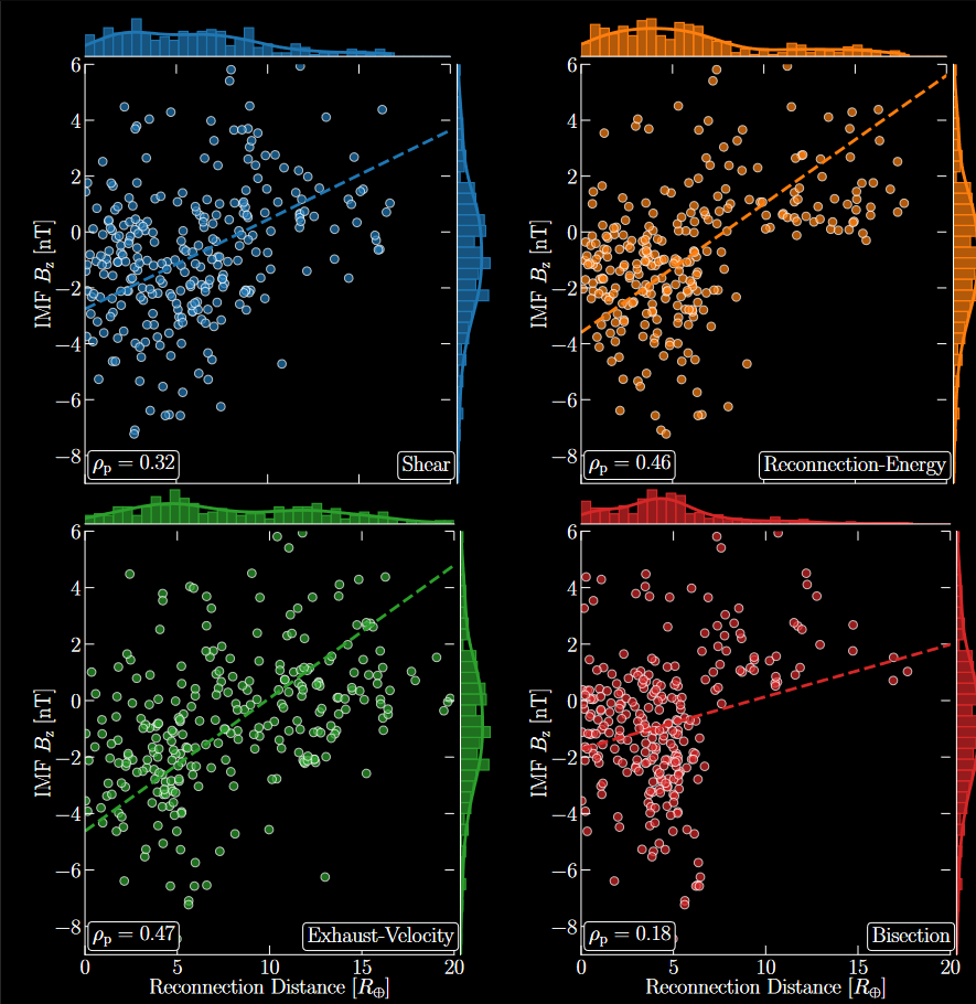
The maximum shear model:
[Qudsi et al., 2023, in Prep]
The maximum exhaust velocity model
[Qudsi et al., 2023, in Prep]
[Qudsi et al., 2023, in Prep]
[Qudsi et al., 2023, in Prep]
[Qudsi et al., 2023, in Prep]
[Qudsi et al., 2023, in Prep]

[Qudsi et al., 2023, in Prep]

[Qudsi et al., 2023, in Prep]
DISCUSSIONS
Qudsi (qudsira@bu.edu)
Discussions:
For negative z-component of IMF, reconnection energy and bisection field models both give very similar statistics.
Maximum Exhaust velocity appears to perform worse than other models. Can be because of poor assumption of ion-density in the magnetosphere.
Statistically, bisection field model seem to perform better than other models for different IMF and magnetopause conditions.
Qudsi (qudsira@bu.edu)
Overall result of the study largely agrees with observations made elsewhere in the literature.
Bisection model is least affected by the direction of IMF as well the dominance of y-component.
Qudsi (qudsira@bu.edu)
Thank You!
Link to the presentation